| Logistic Regression | 您所在的位置:网站首页 › coursera where are complete source code examples › Logistic Regression |
Logistic Regression
|
Logistic regression is a predictive modelling algorithm that is used when the Y variable is binary categorical. That is, it can take only two values like 1 or 0. The goal is to determine a mathematical equation that can be used to predict the probability of event 1. Once the equation is established, it can be used to predict the Y when only the Xs are known. 1. Introduction to Logistic RegressionEarlier you saw what is linear regression and how to use it to predict continuous Y variables. In linear regression the Y variable is always a continuous variable. If suppose, the Y variable was categorical, you cannot use linear regression model it. So what would you do when the Y is a categorical variable with 2 classes? Logistic regression can be used to model and solve such problems, also called as binary classification problems. A key point to note here is that Y can have 2 classes only and not more than that. If Y has more than 2 classes, it would become a multi class classification and you can no longer use the vanilla logistic regression for that. Yet, Logistic regression is a classic predictive modelling technique and still remains a popular choice for modelling binary categorical variables. Another advantage of logistic regression is that it computes a prediction probability score of an event. More on that when you actually start building the models. Building the model and classifying the Y is only half work done. Actually, not even half. Because, the scope of evaluation metrics to judge the efficacy of the model is vast and requires careful judgement to choose the right model. In the next part, I will discuss various evaluation metrics that will help to understand how well the classification model performs from different perspectives. 2. Some real world examples of binary classification problemsYou might wonder what kind of problems you can use logistic regression for. Here are some examples of binary classification problems: Spam Detection : Predicting if an email is Spam or not Credit Card Fraud : Predicting if a given credit card transaction is fraud or not Health : Predicting if a given mass of tissue is benign or malignant Marketing : Predicting if a given user will buy an insurance product or not Banking : Predicting if a customer will default on a loan. 3. Why not linear regression?When the response variable has only 2 possible values, it is desirable to have a model that predicts the value either as 0 or 1 or as a probability score that ranges between 0 and 1. Linear regression does not have this capability. Because, If you use linear regression to model a binary response variable, the resulting model may not restrict the predicted Y values within 0 and 1. 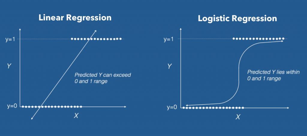 Linear vs Logistic Regression
4. The Logistic Equation
Linear vs Logistic Regression
4. The Logistic Equation
Logistic regression achieves this by taking the log odds of the event ln(P/1?P), where, P is the probability of event. So P always lies between 0 and 1. 
Taking exponent on both sides of the equation gives: Want to become awesome in ML?Hi! I am Selva, and I am excited you are reading this! You can now go from a complete beginner to a Data Science expert, with my end-to-end free Data Science training. No shifting between multiple books and courses. Hop on to the most effective way to becoming the expert. (Includes downloadable notebooks, portfolio projects and exercises) Start free with the first course 'Foundations of Machine Learning' - a well rounded orientation of what the field of ML is all about. Enroll to the Foundations of ML Course (FREE) Sold already? Start with the Complete ML Mastery Path 
You can implement this equation using the glm() function by setting the family argument to "binomial". # Template code # Step 1: Build Logit Model on Training Dataset logitMod $ Cl.thickness : Ord.factor w/ 10 levels "1" Residual Deviance: 243.6 AIC: 263.6In above model, Class is modeled as a function of Cell.shape alone. But note from the output, the Cell.Shape got split into 9 different variables. This is because, since Cell.Shape is stored as a factor variable, glm creates 1 binary variable (a.k.a dummy variable) for each of the 10 categorical level of Cell.Shape. Clearly, from the meaning of Cell.Shape there seems to be some sort of ordering within the categorical levels of Cell.Shape. That is, a cell shape value of 2 is greater than cell shape 1 and so on. This is the case with other variables in the dataset a well. So, its preferable to convert them into numeric variables and remove the id column. Had it been a pure categorical variable with no internal ordering, like, say the sex of the patient, you may leave that variable as a factor itself. # remove id column bc Deviance Residuals: #> Min 1Q Median 3Q Max #> -2.1136 -0.0781 -0.0116 0.0000 3.9883 #> Coefficients: #> Estimate Std. Error z value Pr(>|z|) #> (Intercept) 21.942 3949.431 0.006 0.996 #> Cl.thickness.L 24.279 5428.207 0.004 0.996 #> Cl.thickness.Q 14.068 3609.486 0.004 0.997 #> Cl.thickness.C 5.551 3133.912 0.002 0.999 #> Cl.thickness^4 -2.409 5323.267 0.000 1.000 #> Cl.thickness^5 -4.647 6183.074 -0.001 0.999 #> Cl.thickness^6 -8.684 5221.229 -0.002 0.999 #> Cl.thickness^7 -7.059 3342.140 -0.002 0.998 #> Cl.thickness^8 -2.295 1586.973 -0.001 0.999 #> Cl.thickness^9 -2.356 494.442 -0.005 0.996 #> Cell.size.L 28.330 9300.873 0.003 0.998 #> Cell.size.Q -9.921 6943.858 -0.001 0.999 #> Cell.size.C -6.925 6697.755 -0.001 0.999 #> Cell.size^4 6.348 10195.229 0.001 1.000 #> Cell.size^5 5.373 12153.788 0.000 1.000 #> Cell.size^6 -3.636 10824.940 0.000 1.000 #> Cell.size^7 1.531 8825.361 0.000 1.000 #> Cell.size^8 7.101 8508.873 0.001 0.999 #> Cell.size^9 -1.820 8537.029 0.000 1.000 #> Cell.shape.L 10.884 9826.816 0.001 0.999 #> Cell.shape.Q -4.424 6049.000 -0.001 0.999 #> Cell.shape.C 5.197 6462.608 0.001 0.999 #> Cell.shape^4 12.961 10633.171 0.001 0.999 #> Cell.shape^5 6.114 12095.497 0.001 1.000 #> Cell.shape^6 2.716 11182.902 0.000 1.000 #> Cell.shape^7 3.586 8973.424 0.000 1.000 #> Cell.shape^8 -2.459 6662.174 0.000 1.000 #> Cell.shape^9 -17.783 5811.352 -0.003 0.998 #> (Dispersion parameter for binomial family taken to be 1) #> Null deviance: 465.795 on 335 degrees of freedom #> Residual deviance: 45.952 on 308 degrees of freedom #> AIC: 101.95 #> Number of Fisher Scoring iterations: 21 9. How to Predict on Test DatasetThe logitmod is now built. You can now use it to predict the response on testData. pred 0.5, then it can be classified an event (malignant).So if pred is greater than 0.5, it is malignant else it is benign. y_pred_num 0.5, 1, 0) y_pred |
【本文地址】